Standard Plots
IsoPops implements the following suite of summary plots which may be useful for getting a sense of the isoform diversity in your data. All standard plot functions require the package ggplot2 and take in a processed Database object. These functions also allow for subsetting of the dataset by a list of genes, and most let you toggle between viewing summary statistics for transcripts and/or ORFs.Isoform Length Distributions
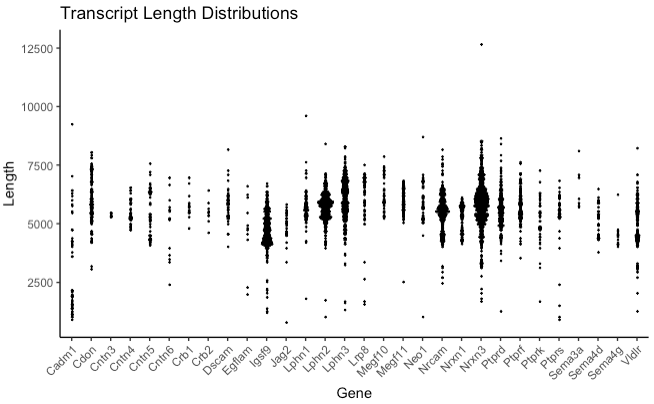
plot_length_dist(database, use_ORFs = F, bins = 200, horiz_spread = 0.3, ...)
Generates a dot plot showing how transcripts/ORFs are distributed in length for each gene in the database.
Arguments
database |
A compiled Database object. |
|---|---|
use_ORFs |
Logical. Set to TRUE to use abundances from OrfDB instead of abundances from TranscriptDB. Note that OrfDB collapses isoforms with non-unique transcripts, so abundances may differ significantly. |
bins |
The number of bins to use in segmenting the range of lengths over the entire dataset. This parameter determines vertical dot spread. |
genes_to_include |
Vector of gene names to subset from the database. Default is to plot all genes in the database. |
horiz_spread |
Numeric. This parameter determines horizontal dot spread across all the genes visualized. |
insert_title |
String to customize the title of the plot. |
Returns
A length distribution dot plot constructed as a ggplot object.Example Usage
                       # database setup
                      gene_ID_table <- data.frame(ID = c("PB.1"), Name = c("Gene1"))
                      rawDB <- compile_raw_db(transcript_file, abundance_file, gff_file, ORF_file)
                      DB <- process_db(rawDB, gene_ID_table)

                      plot_length_dist(DB)
Notes
Requires theggplot2 package.
Treemap Plots
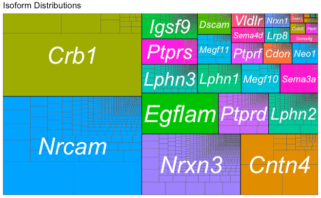
plot_treemap(database, use_ORFs = F, ...)
Generates a treemap plot showing how individual transcripts and genes account for abundance within the dataset as a whole
Arguments
database |
A compiled Database object. |
|---|---|
use_ORFs |
Logical. Set to TRUE to use abundances from OrfDB instead of abundances from TranscriptDB. Note that OrfDB collapses isoforms with non-unique transcripts, so abundances may differ significantly. |
genes_to_include |
Vector of gene names to subset from the database. Default is to plot all genes in the database. |
insert_title |
String to customize the title of the plot. |
Returns
A treemap plot constructed as a ggplot object.Example Usage
                       # database setup
                      gene_ID_table <- data.frame(ID = c("PB.1"), Name = c("Gene1"))
                      rawDB <- compile_raw_db(transcript_file, abundance_file, gff_file, ORF_file)
                      DB <- process_db(rawDB, gene_ID_table)

                      plot_treemap(DB)
Notes
Requires theggplot2 package.
Exon-Abundance Distribution Plots
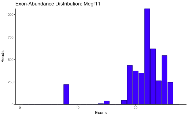
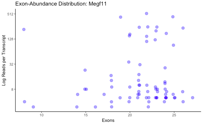
 plot_exon_dist(database,
                           sum_dist = T, bin_width = 0.02, ...)
Generates a bar plot showing the abundances of normalized exon counts for one or more genes. If each transcript is represented as the fraction of exons it contains out of the maximum number of exons found in a gene, this plot is merely a histogram of those representations, weighted by the read count for each transcript. Normalized exon percent is along the x-axis, and abundance is along the y-axis. If only one gene name is given, a second plot is generated where the x-axis is not normalized, instead showing the exon count of each transcript individually, and the y-axis is log-transformed. Jitter along the x-axis is added to improve visibility.
Arguments
database |
A compiled Database object. |
|---|---|
genes_to_include |
Vector of gene names to subset from the database. Default is to plot all genes in the database. |
sum_dist |
Logical. If TRUE, the result is a histogram-like bar plot, where the x-axis is binned. Otherwise, individual isoforms are plotted as points, and the y-axis is log-transformed (single gene only). |
bin_width |
The histogram bin width, used only when multiple genes are input and the x-axis is the fraction of total exons per gene. |
insert_title |
String to customize the title of the plot. |
Returns
A ggplot object.Example Usage
                       # database setup
                      gene_ID_table <- data.frame(ID = c("PB.1"), Name = c("Gene1"))
                      rawDB <- compile_raw_db(transcript_file, abundance_file, gff_file, ORF_file)
                      DB <- process_db(rawDB, gene_ID_table)

                      plot_exon_dist(DB, sum_dist = T)  # set to false for scatter plot
Notes
Requires theggplot2 package.
Unique Isoforms/ORFs Barplots
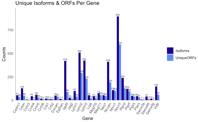
plot_counts(database, use_log = F, use_counts = c("Isoforms", "ORFs"))
Generates a bar plot showing the number of unique isoform transcripts and unique ORFs for each gene.
Arguments
database |
A compiled Database object. |
|---|---|
use_ORFs |
Logical. Set to TRUE to use abundances from OrfDB instead of abundances from TranscriptDB. Note that OrfDB collapses isoforms with non-unique transcripts, so abundances may differ significantly. |
genes_to_include |
Vector of gene names to subset from the database. Default is to plot all genes in the database. |
insert_title |
String to customize the title of the plot. |
Returns
A ggplot object.Example Usage
                       # database setup
                      gene_ID_table <- data.frame(ID = c("PB.1"), Name = c("Gene1"))
                      rawDB <- compile_raw_db(transcript_file, abundance_file, gff_file, ORF_file)
                      DB <- process_db(rawDB, gene_ID_table)

                      plot_N50_N75(DB)
Notes
Requires theggplot2 package.
N50/N75 Barplots
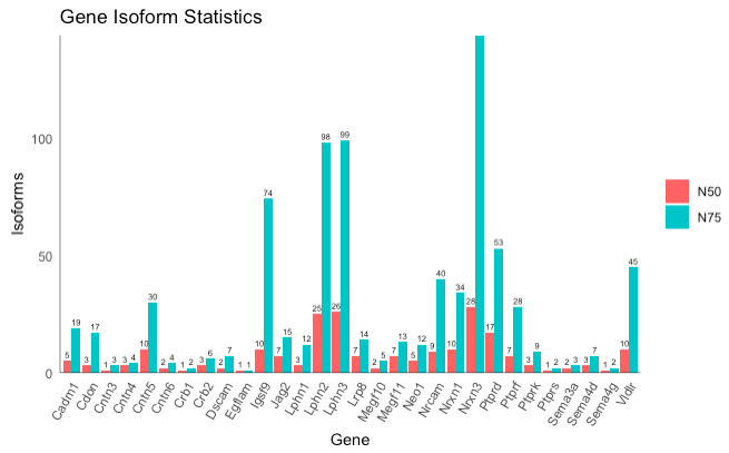
plot_N50_N75(database, use_ORFs = F, ...)
Generates a bar plot showing the number of isoform transcripts and/or unique ORFs for each gene, using the thresholding concepts of N50 and N75. N50 refers to the minimum number of isoforms/ORFs needed to represent at least 50% of the abudance of a gene, while N75 refers to the minimum number of isoforms/ORFs needed to represent at least 75% of the abundance for a gene. This plot can help to identify which genes are dominated by very few isoforms.
Arguments
database |
A compiled Database object. |
|---|---|
use_log |
Logical. If true, y-axis is plotted on a log scale (base 2). |
genes_to_include |
Vector of gene names to subset from the database. Default is to plot all genes in the database. |
use_counts |
One of both of the strings "Isoforms" and "ORFs", indicating which whould be included in the plot. Default is both and to give a warning if no ORF information is in the database. |
insert_title |
String to customize the title of the plot. |
Returns
A ggplot object.Example Usage
                       # database setup
                      gene_ID_table <- data.frame(ID = c("PB.1"), Name = c("Gene1"))
                      rawDB <- compile_raw_db(transcript_file, abundance_file, gff_file, ORF_file)
                      DB <- process_db(rawDB, gene_ID_table)

                      plot_isoform_orf_counts(DB)
Notes
Requires theggplot2 package.
Shannon Diversity Index Plots
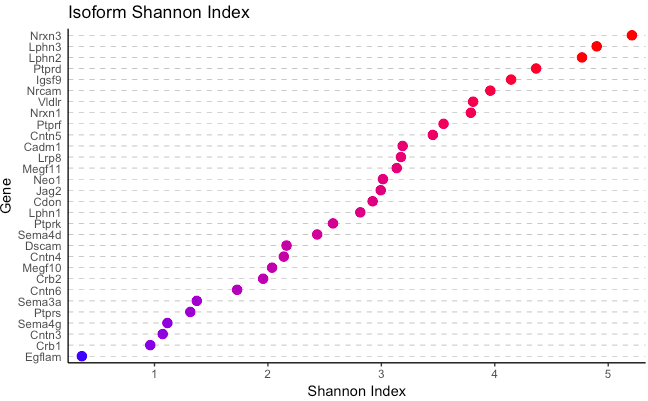
plot_Shannon_index(database, use_ORFs = F, ...)
Generates a plot showing the Shannon Index for isoform/ORF diversity on the x-axis, and each gene on the y-axis.
Arguments
database |
A compiled Database object. |
|---|---|
use_ORFs |
Logical. Set to TRUE to use abundances from OrfDB instead of abundances from TranscriptDB. Note that OrfDB collapses isoforms with non-unique transcripts, so abundances may differ significantly. |
genes_to_include |
Vector of gene names to subset from the database. Default is to plot all genes in the database. |
insert_title |
String to customize the title of the plot. |
Returns
A ggplot object.Example Usage
                       # database setup
                      gene_ID_table <- data.frame(ID = c("PB.1"), Name = c("Gene1"))
                      rawDB <- compile_raw_db(transcript_file, abundance_file, gff_file, ORF_file)
                      DB <- process_db(rawDB, gene_ID_table)

                      plot_Shannon_index(DB)
Notes
Requires theggplot2 package.
Exon Correlation Plots
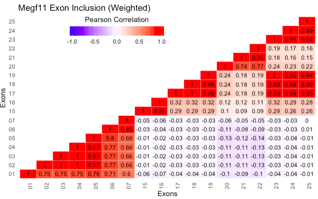
 plot_exon_correlations(database, exon_filename, gene, weighted = T,
                                   exons_to_include = NULL, weights = NULL, plot_hist = F, symmetric = F)
Generates a 2D heatmap where each axis is the exons for a gene, and the values in the heatmap correspond to the correlation between the splicing events of pairs of exons. For example, the heatmap cell in row i and column j contains the pearson correlation of all the observed splicing inclusions and exclusions of exons i and j, according to the transcripts in the data. This plot can show which exons tend to either be included or spliced out together, for instance, and any exon pairs which may have mutually exclusive splicing patterns. Exon presence within a transcript is determined by literal string matching, so only full and completely correct matches between exon sequence and transcript sequence are considered.
Arguments
database |
A compiled Database object. |
|---|---|
exon_filename |
Path to a file in either FASTA or TSV format. If in FASTA format, the sequences are the annotated sequences for all exons in the gene, and the IDs are the exon names (will be displayed in the plot). The ID line must have format ">exonname". If in TSV format, There must be one column for exon names and one column for the exon sequence, tab-separated. |
gene |
The desired gene to plot. Note that the plot will be generated only from exon matches to transcripts for the given gene, so no off-target exon matches are possible. |
weighted |
Logical. If TRUE, transcript abundances will be taken into account when correlations are calculated (recommended). |
exons_to_include |
Vector of exon names to subset from the input file. Default is to include all exons in the inut file. This list is ordered; in other words, if you would like to rearrange the order of exon names on the axes of the heatmap, use this argument to do so. |
weights |
A numeric vector specifying the weights to apply to each transcript for the given gene. Default is the number of full-length reads for the transcript. |
plot_hist |
Logical. If TRUE, a histogram of all exon correlations across the gene is produced. |
symetric |
Logical. If TRUE, both sides of the symmetric heatmap are shown. |
Returns
A ggplot object.Example Usage
                       # database setup
                      gene_ID_table <- data.frame(ID = c("PB.1"), Name = c("Gene1"))
                      rawDB <- compile_raw_db(transcript_file, abundance_file, gff_file, ORF_file)
                      DB <- process_db(rawDB, gene_ID_table)

                      plot_exon_correlations(DB)
Notes
Requires theggplot2 package.