Visualizing Isoform Populations with PCA or t-SNE

To interpret the isoform diversity in your data, it can be helpful to view the "spread" or "distribution" of transcripts for one or more genes in a low-dimensional setting. IsoPops can perform dimension reduction followed by visualization using either PCA or t-SNE, two popular unsupervised machine learning tools. The resulting plots display isoforms such that more similar isoforms are close to each other, while more divergent isoforms are farther away from one another. The process for generating these plots is:

1. Quantitatively represent transcript (or ORF) sequences as vectors via gene-agnostic, annotation-agnostic k-mer counting.
2. Run either PCA or t-SNE on these vectorized representations of isoforms.
3. Plot the PCA or t-SNE embeddings of the isoforms, in 2D or 3D.

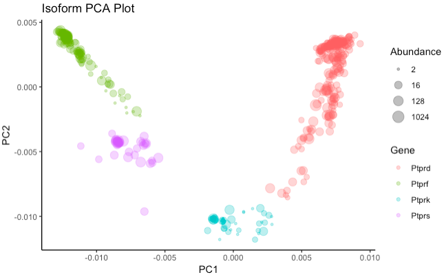
These three steps are each performed with a single function call in IsoPops, as shown below:

                    counts <- get_kmer_counts(DB, genes = c("Ptprd", "Ptprf", "Ptprk", "Ptprs"))
                    pca <- kmer_PCA(DB, counts)
                    plot_PCA(DB, pca)
                  

To plot in 3D, replace the last line with plot_3D_PCA(DB, pca).

To run t-SNE instead:

                    counts <- get_kmer_counts(DB, genes = c("Ptprd", "Ptprf", "Ptprk", "Ptprs"))
                    tsne <- kmer_tSNE(DB, counts, iterations = 5000, perplexity = 40, dims = 2)
                    plot_tSNE(DB, tsne)
                  

To plot in 3D:

                    counts <- get_kmer_counts(DB, genes = c("Ptprd", "Ptprf", "Ptprk", "Ptprs"))
                    tsne3D <- kmer_tSNE(DB, counts, dims = 3)
                    plot_tSNE(DB, tsne3D, force_3D = T)
                  

To generate these plots using ORF sequences instead of transcript sequences, simply add the argument use_ORFs = T to each function (including the plot functions).